Code
1. Goal
The problem setting is to solve the Acrobot problem in OpenAI gym. The acrobot system includes two joints and two links, where the joint between the two links is actuated. Initially, the links are hanging downwards, and the goal is to swing the end of the lower link up to a given height (the black horizontal line)

2. Environment
The acrobot environment has a continuous state space as follows (copied from source code comments):
State:
The state consists of the sin() and cos() of the two rotational joint angles and the joint angular velocities :
\[[\cos(\theta_1), \sin(\theta_1), \cos(\theta_2), \sin(\theta_2), v_1,v_2]\]For the first link, an angle of 0 corresponds to the link pointing downwards. The angle of the second link is relative to the angle of the first link.
For example:
- an angle of 0 corresponds to having the same angle between the two links.
- a state of [1, 0, 1, 0, …, …] means that both links point downwards.
Action:
The action is either applying +1, 0 or -1 torque on the joint between the two pendulum links.
Reward:
At each timestep (not episode), the reward is set to be -1 if the lower end never reaches the horizontal ruler, and 0 if it has.
Terminal Condition:
The environment imposes a 500 timestep limit to each episode, which means after 500 timesteps, if the pole still hasn’t reached the goal, the episode will terminate and reset.
Solved Condition:
There are no specific requirements, see the experiments section for a comparison of performance with the leaderboard.
3. Approach
3.1 Algorithm Comparison
I chose to use actor-critic with state-value temporal difference (TD) to train an on-policy agent. I assumed an infinite time horizon when deciding on the algorithm, since this problem requires the agent to build momentum to actually swing up to the top, which means the policy can’t be short-sighted and needs to consider all the actions it took to build momentum and finally reach the goal.
Key considerations:
- The state space is continuous, it would be inefficient to represent the state-action values (q-values) in traditional tabular form.
- This problem does not require a global optimal solution, we consider the problem solved after reaching a reward of larger than -100. This means that we can trade-off the accuracy of the algorithm in exchange for a more efficient training process while still finding a near-global optimal policy.
- Dense rewards. There is no final reward, rather the reward is given at every time step, and represents how far/close the agent is from the goal, so the feedback is very “real-time”.
- If the problem is using an on-policy algorithm, then we should consider adding temporal difference (baseline) to reduce the variance of the gradient estimation while ensuring the bias is not increased.
3.2 Problem Parameterization
I initially started with simple radial-basis functions with 10 centers for each of the state dimensions, which resulted in \(10^6\) size state space. This drastically slowed down the training of my agent and the progress of this project, so I switched to use a neural network to parameterize both the value function and policy function.
Key considerations:
Since this problem is in a continuous space, I had to use a function approximator to approximate the state space which can then be used to train the agent.
3.3 Policy
I initially attempted to use a Gaussian function with varying \(\sigma\), but it was very inefficient and ineffective to hand-tweak the \(\sigma\) and parameterize the Gaussian mean, so I eventually resorted to a neural network.
Key consideration:
The relationship between actions and state space is non-linear
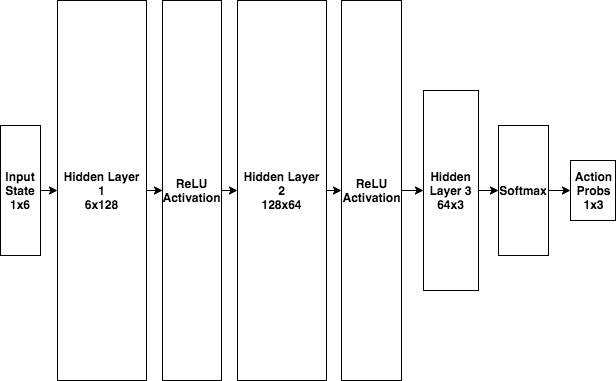
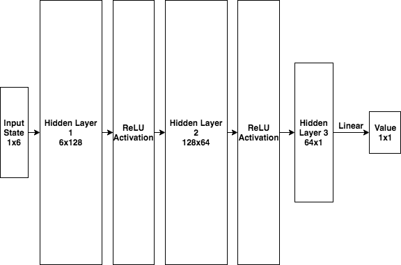
3.4 Neural Network Architecture
By incorporating the Rectified-Linear unit (ReLU) activation function, we can represent the non-linear relationship between the state space, the policy, and the value of that state. Please refer to [4.3 Neural Network Complexity] section for the reasoning behind the number of neurons.
3.5 Hyperparameters
- Actor’s (Policy) Learning Rate (\(\alpha_{a}\)): \(1 \times 10^{-4}\)
- Critic’s (Value) Learning Rate (\(\alpha_{c}\)): \(5 \times 10^{-3}\)
- Discount Rate (\(\gamma\)): 0.9
- Neural Network Weight Initialization: Normal Distribution with zero mean and 0.1 standard deviation
- Neural Network Bias Initialization: 0.1 constant
- 128/64 Neurons in the first/second hidden layer respectively for both the policy network and the value network
4. Experiment & Findings
4.1 Performance
| User | Best 100-episode performance |
|---|---|
| mallochio | -42.37 ± 4.83 |
| marunowskia | -59.31 ± 1.23 |
| MontrealAI | -60.82 ± 0.06 |
| BS Haney | -61.8 |
| Felix Nica | -63.13 ± 2.65 |
| Daniel Barbosa | -67.18 |
| Mahmood Khordoo | -68.63 |
| lirnli | -72.09 ± 1.15 |
| Tiger37 | -74.49 ± 10.87 |
| tsdaemon | -77.87 ± 1.54 |
| a7b23 | -80.68 ± 1.18 |
| DaveLeongSingapore | -84.02 ± 1.46 |
| Sanket Thakur | -89.29 |
| loicmarie | -99.18 ± 2.60 |
| simonoso | -113.66 ± 5.15 |
| alebac | -427.26 ± 15.02 |
| mehdimerai | -500.00 ± 0.00 |
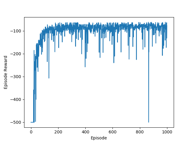
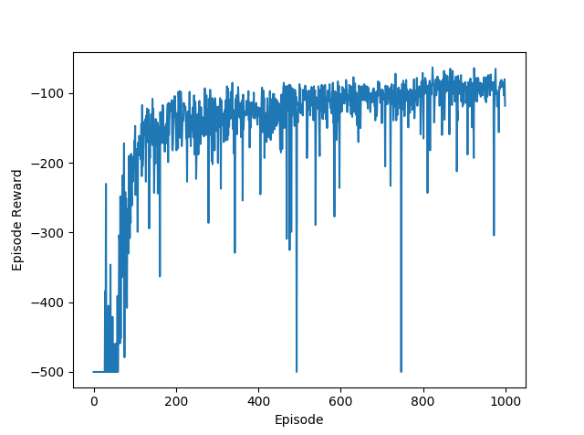
Compared to the leaderboard, our last 100 episode (total 1000 episodes) average reward is -74.9, with raw rewards below:
EP[150]: -275.0
EP[160]: -231.0
EP[170]: -243.0
EP[180]: -209.0
EP[190]: -277.0
EP[200]: -268.0
EP[210]: -357.0
EP[220]: -115.0
EP[230]: -101.0
EP[240]: -98.0
EP[250]: -141.0
EP[260]: -86.0
...
EP[910]: -83.0
EP[920]: -77.0
EP[930]: -70.0
EP[940]: -80.0
EP[950]: -80.0
EP[960]: -132.0
EP[980]: -82.0
EP[990]: -76.0
EP[1000]: -69.0
This shows that with a baseline agent, with only a simple 2-layer neural network to approximate the policy and value functions, the performance is relatively good (about average on the leaderboard). The agent is also able to reach > -200 rewards at around 220 episodes and convergences to > -100 rewards after 240 episodes. The next section will depict the reward/episode relationship, which shows the fast convergence of this algorithm.
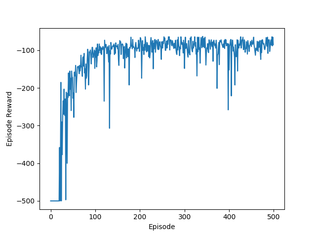
4.2 Training Duration
| # Episodes | Training Time | Avg Reward (last 100 episodes) |
|---|---|---|
| 1000 | 404 seconds | -74.9 |
| 500 | 256 seconds | -82.3 |
| 250 | 151 seconds | -90.5 |
We can see that even with 500 episodes of training, the agent is able to converge to > -100 rewards at around 60 episodes. The table shows that, with this approach, training for 500 episodes is sufficient for a baseline performance, and further training has only marginal gains in terms of improving average reward. Perhaps, this shows that performance could be bottlenecked by our simple 2-layer neural network’s function approximation ability.
4.3 Neural Network Complexity
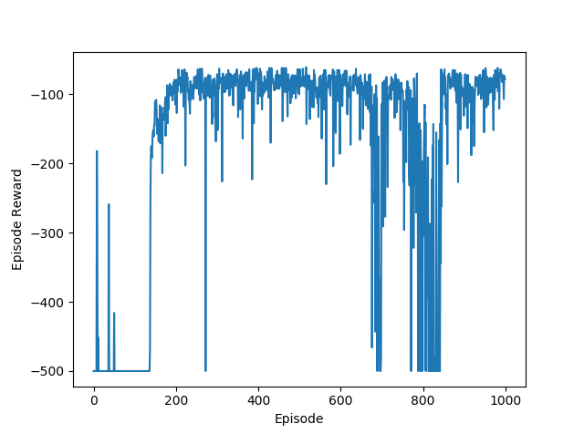
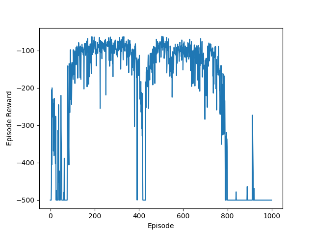
If we have too many neurons per layer, it will likely to overfit the function, whether that’s the value function or the policy. Translated into rewards, the neural network will try to learn a more complex value function and policy, where in reality, the “true” function is not that complex, resulting in the agent taking worse actions, and leading to the big gaps and unstable rewards, shown in in the 128/256 neuron case. If we have too few neurons, such as 32 and 16 in layer1 and layer2 respectively, the neural network will not be complex enough to approximate the value function and the policy, which is reflected in the first plot, showing slower learning and more variance in the reward/episode. The best number of neurons is 128 and 64 in layer1 and layer2 respectively, shown in the second plot.
4.4 Discount Rate
No Discount Rate
With Discount Rate
Since I assumed the algorithm to be operating in infinite time horizon, adding in a discount rate helps with the reward estimation. Intuitively, the task of reaching the goal can be accomplished within a couple of timesteps, but during the training process, the agent will accumulate a lot of failed attempts in building momentum. Without a discount rate, these failed attempts will be will be equally weighted when computing the value for this episode.
5. Next Steps
Since we’re using a simple neural network to represent both the policy and value function for our actor-critic algorithm, there could be potential improvements if we increase the complexity of these networks. Perhaps, with a more complex non-linear function approximator, there could be improvement in performance. At the same time, training for a longer period might be necessary to fully adjust the weights of the neural network.
It is always a good thing to try out other value functions such as deep Q-learning, combined with the actor-critic approach.