Creating Neural Networks with Python/Keras/Tensorflow to Predict the Future

Previous Knowledge Required

Understand what is a neural network (NN) and how it works conceptually.
Python
Basic understanding of what derivatives/gradients are

Goals

In this tutorial, I will go over 3 different approaches of creating a NN that can predict the prices of a particular cryptocurrency pair (ETHBTC). This include using (very-low-level) Numpy/raw Python, (low-level) Tensorflow and (high-level) Keras.

Since it’s similar to predicting any price/number given a sequence of historical prices/numbers, I will describe this process as general as possible. The purpose of this tutorial is more about how to create NNs from scratch and to understand how high level frameworks like Keras work underneath the hood. It’s less about the correctness of predicting the future.

Personal goal: When I was studying machine learning, I thought it would be good for me to implement things at the low level first, and then slowly move up the abstraction to improve productivity. I made sure that the 3 approaches all achieved the same outcome.

Showcase

Since the outcome of the 3 approaches are the same, I’ll just show one set of the training and testing result. All three sets are in the repo, and you can regenerate them if you’d like.

Note: The prices in the graph are normalized, but the accuracy is the same if denormalized. Again, this is just an illustration of how NN works and by no means a correct way to predict prices.

Training Set

Test Set

Input Data

82 Hours worth of BTCETH data in 10-second increments covering the following dimensions:

Closing price
high
low
volume

Source: Binance

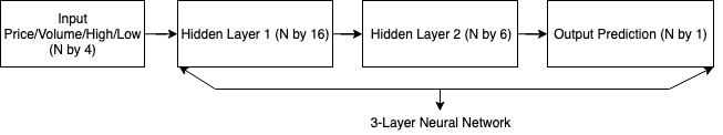
Neural Network Architecture (All 3 Versions)

3 Layers, Relu Activation Function for first (n-1) layers, with last layer being a linear output. The 1st hidden layer contains 16 neurons, the 2nd hidden layer contains 6 neurons. The N denotes the number of samples.

Note that when counting layers, we usually don’t count the layer without tunable parameters. In this case, the input layer doesn’t have tunable parameters, which results in a 3-layer NN, as opposed to a 4-layer NN.

Version 1

(Hand-coded Neural Network (without using any 3rd party framework)

Code

In this version, we need to understand the innerworkings of NNs. In other words, how propagation of neuron computations take place and how to compute gradients from a programmatic perspective. I’ve borrowed and adapted some of the homework code from Andrew Ng’s Coursera Course on Deep Learning and Neural Networks to fit our context.

1. Initialize parameters

Neuron Weights (W)
Bias Weights (B)

2. Define hyperparameters

Learning Rate - how much each step of gradient descent should move
Number of training iterations
Number of hidden layers (Layers excluding input layer)
Activation function for each layer

The dimensions of the NN is defined on this line: layers_dims = [X_train.shape[0], 16, 6, Y_train.shape[0]]

It means the first input layer takes in a size of X_train.shape[0]. In our example, that would be equal to 4 since there are 4 dimensions (Price, High, Low, Volume) for every data point. The first hidden layer (2nd element in the array) contains 16 neurons, second hidden layer contains 6 neurons, and the output layer contains Y_train.shape[0], in our example that is equal to 1 since we’re predicting one price at a time.

To summarize, the NN looks like this

3. Define and perform training - loop for num_iterations:

Forward propagation

  Usually one forward pass goes like this:

  Input -> Matrix Multiplication (Linear) -> Activation Function (Non-Linear)-> 
  |_____________________ Repeat this N times (N Layers) ______________________|

In our price prediction example (we use a linear output since we’re predicting values not classifying categories): [LINEAR->RELU]*(N-1)->LINEAR

  Matrix Multiplication (Linear) = Input X * Weights + Bias
  Activation Function (Non-Linear) = Relu(Matrix Multiplication Result) = max(0, result)

Compute cost function

After we have performed one pass of our forward propagation, we will have obtained the predictions (from the last layer’s activation function output) and we can compare it with the ground truth to compute the cost. Note that I’m using MSE (Mean-squared Error), that’s a common cost function for value prediction. I’ll keep the notations consistent with the code so you can refer to it if necessary.
```
  AL -- predicted "values" vector, shape (1, number of examples)
  Y -- true "values" vector, shape (1, number of examples)

  cost = (np.square(AL - Y)).mean(axis=1)
```
Backward propagation

After computing the cost, or how far off our predictions are from our true values, we can use that cost to adjust our weights in our NN. But first, we need to get the gradients of 3 things with respect to our cost: (1) Gradient of predicted Y value, (2) gradient of weights of each hidden unit, and (3) gradient of weights of the bias unit. With these gradients under our belt, we can know how to adjust our weights to minimize the cost.
```
  One backward pass goes like this, the 3 gradients will be computed for each layer

  Cost ->  Activation Function (Non-Linear)-> Matrix Multiplication (Linear) ->
  |_____________________ Repeat this N times (N Layers) ______________________|
```
Update parameters (using parameters, and grads from backprop)

At this stage, we have finished one back propagation and obtained all 3 types of gradients for all of our weights needed to adjust our NN.
```
  parameters["W" + str(l + 1)] = parameters["W" + str(l + 1)] - learning_rate * grads["dW" + str(l + 1)]
  parameters["b" + str(l + 1)] = parameters["b" + str(l + 1)] - learning_rate * grads["db" + str(l + 1)]
```
We’re simply doing:

parameter = parameter - learning rate * gradient of that parameter

4. Use trained parameters to predict prices

We just perform a forward pass just like in training. It will produce the predicted values based on the current NN weights.

Version 2

Keras-based Neural Network

Code

In this version, since we’re dealing with high-level Keras framework, we only need to have good idea of the architecture of the NN and how to construct it using the building blocks provided by Keras (just like lego). We don’t need to implement matrix multiplication or activation functions. We should, however, understand how we initialize our weights, which activation functions to choose and how to structure our NN. If you have time, you might even want to tweak the “icing on the cake” to prevent overfitting by applying regularization and dropout techniques. The reason I mention the “icing” here in version 2 and not in version 1 is because all of these components are lego pieces that you don’t need to implement yourself. This is why high-level frameworks provide a productivity boost over hand-coded solutions. But it’s always good to understand what’s going on under the hood to debug potential issues.

In our example:

Instantiate a sequential model. This is like a container that holds the NN and its layers. Read more about Keras Sequential Models

model = Sequential()
Add a Layer to the NN, note that we don’t need separate functions for forward/backward propagation, we just think in terms of layers in the NN. Read more about Keras Layers. The 16 is the number of neurons in this layer, and we’re using relu as the activation function. Remember the building block argument I said before, in a high-level framework, we only need to determine what pieces we need to build the NN, as opposed to implementing them.

model.add(Dense(16, input_dim=X_train.shape[1], activation='relu'))

Note that this is equivalent to our L_model_forward() function and L_model_backward() combined in Version 1 since we think in terms of operations in Version 1, and layers in Version 2
Similarly, we add another layer to the NN. The output space is N by 6 dimenions, where N is the number of samples, and the 6 is the number of neurons in this layer.

model.add(Dense(6, activation='relu'))
Finally, we add our output layer to the NN. The output space (Y_train.shape[1]) in our example is 1, since we’re only predicting one price at a time.

The difference in using .shape[1] and shape[0] in the two versions is because in version 1, to follow Andrew Ng’s course notation, the samples are placed along columns shape[1] and the features (input/output dimension) are rows shape[0]. But in version 2, it’s the opposite, thus Y_train.shape[1] here denotes the output dimension.

model.add(Dense(Y_train.shape[1]))
After the network is fully constructed, we have to tell it how to train the NN. This involves specifying the optimizer for the NN as well as the loss function

model.compile(optimizer=SGD(lr=0.03), loss='mse') # SGD = Stochastic Gradient Descent

Version 3

Tensorflow-based Neural Network

Code

So we’ve seen creating operations from scratch in our Version 1, and using a high-level framework to create a “model” of our NN and just “fitting” it in Version 2. In Version 3, we have to switch our conceptual model of a NN a little bit again, because I have to introduce you to the concept of a Tensor. In my definition, it’s a wrapper or a building block that can encompass a variable, a constant, an operation, or any series of operations. We can connect tensors together by referencing them.

Let’s quickly go through our example and I’ll explain line by line with respect to how they relate to our Version 1 and Version 2 conceptual models.

We will start by defining our input variables:
```
 input_x = tf.placeholder('float', [None, X_train_orig.shape[1]], name='input_x')
 input_y = tf.placeholder('float', [None, Y_train_orig.shape[1]], name='input_y')
```
Note that this is a “placeholder”, which means before we feed in the actual input data, this tensor will be empty. The dimensions for this placeholder is None by X/Y_train_orig.shape[1], this means it’s “any number of samples by shape[1] of features per sample”. The name is optional, but it helps later when we need to debug.

The row/column vs samples/features notations are consistent with Version 2, where shape[1](columns) are the features, and shape[0](rows) are the samples
Next, we will define some of the weights of our NN, namely our hidden unit weights and bias unit weights.
```
 W1 = tf.Variable(tf.random_normal([X_train_orig.shape[1], 16]))
 B1 = tf.Variable(tf.zeros([16]))
```
Note that these tensor types are “Variable”, which means they will “vary” during our training process. These are, by default, trainable variables.
We will define our linear function and activation function together in one line:

layer1 = tf.nn.relu(tf.add(tf.matmul(input_x, W1), B1))

I will leave out the definition for layer2 and output layer since they are similar in nature.

If we break this down and see each computation clearly, it’s equivalent to:
```
 # Matrix Multiplication to get the linear result first

 mat_result = tf.matmul(input_x, W1)
	
 # Add the result to the bias units using Numpy broadcasting

 linear_result = tf.add(mat_result, B1)

 # Apply rectified linear unit activation to the linear function result

 layer1 = tf.nn.relu(linear_result)
```
This is similar to our Version 1 definition, here. Note that we’re refering W1 and B1 varibles from our second step. This establishes the connection between tensors.
Before we can train the network, we still need to define the loss functions and define how to optimize (train) it.
```
 cost = tf.reduce_mean(tf.square(output - input_y))
 optimizer = tf.train.AdamOptimizer(learning_rate=learning_rate).minimize(cost)
```
Note that we’re still reference other tensors output, input_y, and cost. We can use the tf.reduce_mean() function to compute the MSE loss. And since Tensorflow has a built-in AdamOptimizer, we can just call it. This is similar to Version 2’s optimizer=SGD().
Now we have finished defining all the tensors. It’s time to actually feed in the input data and see how the data flow through all the connected tensors.

Initialize all the variables that are not placeholders, such as weights and biases

init = tf.global_variables_initializer()

Feed in our batch_x and batch_y inputs to the placeholders. Note that the names (keys) must match the variable names input_x/y and specify what we want to be returned: optimizer, and cost from step (4).
```
 _, c = sess.run([optimizer, cost], feed_dict={
         input_x: batch_x, 
         input_y: batch_y, 
     })
```

Image from https://playground.tensorflow.org/

As you can see now, after we feed in the input data into the NN, all the connected tensors will subsequently receive the input from the previous output and perform their computations accordingly, thus the name “TensorFlow”.

I will be posting another note for applying reinforcement learning to trading. Since even with predicted prices, the agent will still not know when to buy or sell (i.e. after a 1% price drop? 2%?). We don’t want to hard-code those conditions, rather we want the agent to learn them as the “policy”. Until next time…Thanks!