The A3C method in Reinforcement Learning (RL) combines both a critic’s value function (how good a state is) and an actor’s policy (a set of action probability for a given state). I promise this explanation doesn’t not contain greek letters or calculus. It only contains English alphabets and subtraction in math.
Taken from “Hands-On Reinforcement Learning with Python by Sudharsan Ravichandiran”
Advantage in A3C is used to determine which actions were “good” and “bad”, and it is updated to encourage or discourage accordingly. Note that this also informs the agent how much better it is than expected. This is better than just using discounted rewards in vanilla Deep Q-learning. To see why, below is a formal explanation.
The advantage is estimated using discounted rewards (R) and the value from the critic’s value function, how good a state is, V(s). Thus formally:
Estimated Advantage = R-V(s)
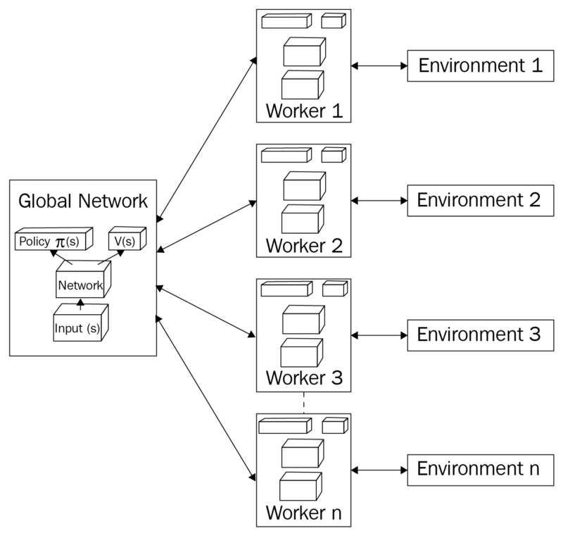
In A3C, there is a global network. This network will consist of a neural network to process the input data (states), and the output layers consists of value (how good a state is) and policy (a set of action probability for a given state) estimations.
The following summarizes the process of each episode:
- To start the process, each worker initializes its network parameters equal to the global network.
- Each worker interacts with its own environment and accumulates experience in the form of tuples (observation, action, reward, done, value) after every interaction.
- Once the worker’s experience history reaches our set size, we calculate the discounted return -> estimated advantage -> temporal difference (TD) ->value and policy losses. Note that we also calculate an entropy of the policy to understand the spread of the action probabilities. In other words, a high entropy is the result of similar action probabilities, or uncertain what to do in laymens terms. A low entropy means the agent is very confident (high probability of one action versus the rest) in the action it choses.
- Once we’ve obtained the value and policy losses from (3), our forward pass (propagation) through the network is complete. Now it’s time for the backward pass (propagation). Each worker uses these calculated losses to compute the gradients for its network parameters.
- We then use the gradients from (4) to update the global network parameters. This is when we reap the benefits of the asynchronous workers. The global network is constantly updated by each worker as they interact with its own environment. The intuition here is that because each worker has it’s own environment, the overall experience for training is more diverse.
- This concludes one round-trip (episode) of training. Then it repeats (1–5)
Overall, the value estimates from the critic is used to update the policy in the actor, which works better than traditional policy gradient methods which doesn’t have a value etimate and solely tries to optimize the policy function. Therefore, it may be intuitive to let the critic learn faster (higher learning rate) than the actor.