- Motivation and Goals
- Abstraction layers of Machine Learning Libraries
- Comparing this project to PyTorch for the same functionality
- Efficiency vs Learning
- Technical Design
- Additional Thoughts
Project link: https://github.com/workofart/ml-by-hand
I recently started working on a project called ML by Hand, which is a machine learning library that I built using just Python and NumPy. Afterwards, I trained various models (classical ones like CNN, ResNet, RNN, LSTM, and more modern architectures like Transformers and GPT) using this library. The motivation came from my curiosity about how to build deep learning models from scratch, like literally from mathematical formulas. The purpose of this project is definitely not to replace the machine learning libraries out there (e.g. PyTorch, TensorFlow), but rather to provide educational material to develop a deeper understanding of how models and libraries are created from scratch. Therefore, our top priority is not to develop the most efficient library, but still good enough to train GPT models locally. The library implementation ensures that code and documentation are explicit enough to illustrate mathematical formulas in its rawest form. This project took inspiration from Micrograd by Andrej Karpathy. I was initially interested in creating just an autograd engine (wikipedia) but this project slowly evolved into a full-fledged machine learning library. Oh well, here we go. 😁
This blog post is structured into several sections. We start by discussing the motivation. Then we move on to understanding the different abstraction layers in machine learning libraries. At this point, we can see where this project fits into the bigger picture. We then compare this project to PyTorch to illustrate my motivation concretely. The bulk of the blog post is centralized around the Technical Design, where we discuss the core components of the library. Finally, I have some additional thoughts while working on this project.
Motivation and Goals
- The goal is for learning (fewer abstractions and closer to math), not for replacing major machine learning libraries
- Learn from first principles (calculus and linear algebra) and express them in their rawest form in code
- Implement techniques and model architectures from academic papers (examples)
- Strip down the abstraction layers of machine learning libraries to understand what’s going on underneath the hood
- Learn to create a machine learning library from scratch
Abstraction layers of Machine Learning Libraries
Below is an illustration of abstraction layers from the highest level to the lowest level.
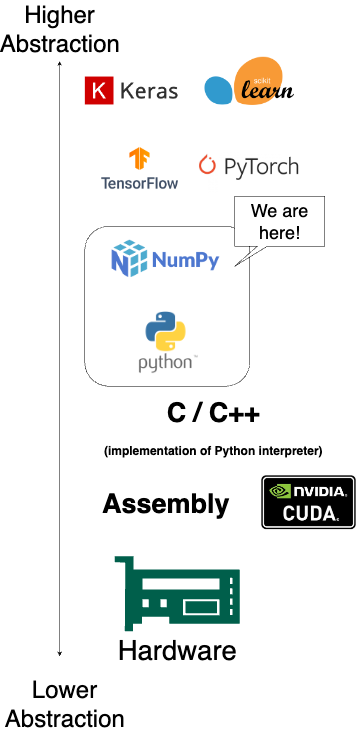
This project operates around the middle layer, which means that we’re basically converting these mathematical formulas from textbooks and papers into NumPy or Python code. I believe that this layer provides the most transparency to show how everything works, yet not so low-level that you’re worried about how the hardware works (another domain). And given that Python is a very beginner-friendly programming language, we want to use this as the starting point.
Comparing this project to PyTorch for the same functionality
Here we are comparing the same functionality in our own library versus PyTorch. Although PyTorch’s APIs are very easy to understand, I think the difference comes in when we want to debug something. So if you want to trace down this function call hierarchy, you can see that PyTorch wraps a lot of functions around, mostly to improve efficiency, but also to be very generic. In our library, we can easily just step through the function call references to see what exactly is happening. And most likely the depth of these function references is about 2 to 3 layers, whereas PyTorch has significant deeper layers.
Let’s try to step through a typical ReLU function in PyTorch.
# Source: https://github.com/pytorch/pytorch/blob/v2.6.0/torch/nn/functional.py#L1693
def relu(input: Tensor, inplace: bool = False) -> Tensor:  # noqa: D400,D402
    """
    Applies the rectified linear unit function element-wise. See
    :class:`~torch.nn.ReLU` for more details.
    """
    if has_torch_function_unary(input):
        return handle_torch_function(relu, (input,), input, inplace=inplace)
    if inplace:
        result = torch.relu_(input)
    else:
        result = torch.relu(input)
    return result
Now, you’re wondering, what’s has_torch_function_unary above? Let’s ignore that and take a look at torch.nn.ReLU as the code comment suggested.
# Source: https://github.com/pytorch/pytorch/blob/9ea1823f96690b4f8b3d79e01c477b3629eab3b6/torch/nn/modules/activation.py#L97
class ReLU(Module):
    r"""Applies the rectified linear unit function element-wise.
    :math:`\text{ReLU}(x) = (x)^+ = \max(0, x)`
    """

    __constants__ = ["inplace"]
    inplace: bool

    def __init__(self, inplace: bool = False):
        super().__init__()
        self.inplace = inplace

    def forward(self, input: Tensor) -> Tensor:
        return F.relu(input, inplace=self.inplace)

    def extra_repr(self) -> str:
        inplace_str = "inplace=True" if self.inplace else ""
        return inplace_str
Ok, so we have the math formula for this ReLU operation in the code comment, which is helpful. But the code implementation is still not found. Let’s trace through the F.relu() function. Wait, that’s referencing something not easily navigable through the IDE. I did some searching and found that the actual implementation of the ReLU function is done in C++. Below is how it’s currently defined, though the exact function signatures or file locations may change in future PyTorch versions.
// Source: https://github.com/pytorch/pytorch/blob/9ea1823f96690b4f8b3d79e01c477b3629eab3b6/aten/src/ATen/native/Activation.cpp#L512-L515
Tensor relu(const Tensor & self) {
  TORCH_CHECK(self.scalar_type() != at::kBool, "Boolean inputs not supported for relu");
  return at::clamp_min(self, 0);
}
So we finally found the code implementation for the ReLU activation function, in terms of math, which is \(\max(0, x)\). But if we want to find the backward (derivative of this formula), that’s another journey. But you get the point now. To be clear, PyTorch is much more efficient than our library because of those additional layers. And that’s the trade-off we’re making here. We’re targeting educational value over efficiency.
Let’s do the same exercise using our library. If we look up the relu function, we first find this wrapper function
# Source: https://github.com/workofart/ml-by-hand/blob/3cf1d45ec2c451af58da2d2b839b1c17fdc0cb9d/autograd/functional.py#L17
def relu(x: Tensor) -> Tensor:
    """
    Applies the Rectified Linear Unit (ReLU) activation function.
    """
    return Relu.apply(x)
Now let’s navigate to Relu class. It’s defined in the same functional.py module.
# source: https://github.com/workofart/ml-by-hand/blob/3cf1d45ec2c451af58da2d2b839b1c17fdc0cb9d/autograd/functional.py#L87
class Relu(Function):
    """
    Rectified Linear Unit (ReLU) activation function.

    The ReLU function is defined as:
        $$
        ReLU(x) = max(0, x)
        $$
    """

    def forward(self, x: np.ndarray) -> np.ndarray:
        self.x = x
        return np.maximum(x, 0)

    def backward(self, grad: Tensor) -> np.ndarray:
        return grad.data * (self.x > 0)
Here we can exactly see the forward function and the backward function. And these correspond exactly to the mathematical formulations of ReLU \(\max(0, x)\) and
\[\frac{\partial{ReLU(x)}}{\partial x} = \begin{cases} 1 & \text{if } x > 0 \\ 0 & \text{if } x \leq 0 \end{cases}\]The forward function is calling NumPy maximum(). And the backward function is performing a simple conditional multiply on a NumPy array self.x and grad.data. There’s nothing too complex about it.
In this project, we intentionally keep the explicit mathematical formulas as shallow as possible so you can easily trace each step and understand why certain functions might fail. You can set breakpoints to debug your model training process without getting lost in multiple abstraction layers. Stepping back, while high-level libraries like PyTorch offer efficiency and extensive functionality, I personally find them less beginner-friendly. That’s why I’m building this project from scratch to bring the code and math closer together so we can connect the dots more easily, without the extra mental load of navigating countless functions and abstraction layers.
Efficiency vs Learning
As mentioned above, this project is not targeted towards efficiency, but rather learning. Therefore, the scope and the nature of the project mean we can only achieve a certain degree of efficiency. After that point, it’s beyond the scope of this project to further optimize at lower levels of abstraction (e.g. C/C++ or kernel level). That being said, the code is still optimized to a certain extent without destroying the educational value and simplicity. I will talk about this later in the technical design section. (spoiler alert: there are a lot of ways to implement the computational graph and depending on which way we do that, there are some efficiency gains both in terms of CPU cycles and memory usage. The wrapper function for ReLU in the above example is part of that).
Along the way, I noticed one low-hanging fruit for efficiency improvement (drop-in replacement for NumPy) – CuPy. This library allows us to enable GPU acceleration with near-zero code changes (hardware-agnostic code). In the animated gif above, I have trained the GPT-2 model on a single GPU accelerated by CuPy. The fundamental acceleration comes from the matrix operations in NumPy -> CuPy, where it could be done in parallel on GPUs, because CuPy has implemented the lower layers of abstraction to talk to the CUDA kernel directly.
As hardware and training technique evolve, we might still be able to achieve great performance on certain datasets, but just a bit behind due to this trade-off. That’s totally fine. The motivation of this project is to understand how models are built from scratch. After we’ve grasped that, we can implement the same model using more efficient libraries such as PyTorch.
Technical Design
This section goes in depth on the various components that make up this machine learning library and how I initially designed these components to interact with each other nicely and in a very easy-to-digest manner.
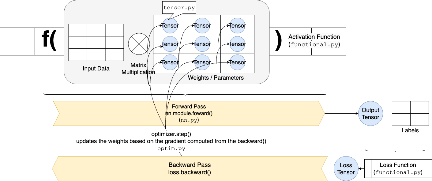
Figure 1
From a 30,000-foot view, you need to provide “Input Data” and “Labels”. Then you can define a neural network using nn.py module. The basic data structure is called a Tensor, which represents things like neural network weights, output as well as loss. Neural networks in nn.py are functions, just like activation and loss functions in functional.py. All functions implement the forward() and backward() interface. The optimizer in optim.py determines how we update our weights. That’s it. Now let’s take a deeper look at each component to understand how everything works.
Tensor Class
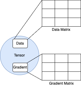
Figure 2
Let’s first introduce the smallest unit of data structure in our library, which is called a Tensor. This data structure basically encapsulates the data as well as the gradient. So those are two main attributes for a tensor. Obviously the data and the gradient are represented by the NumPy arrays. But a lot of our mathematical operations such as adding, subtracting, matrix multiplication are done on the Tensor level. So this means that we need to implement these mathematical operations in the Tensor class.
Tensor-level Operations
The main categories of Tensor operations:
- Binary operations (Add, mul etc…): These operations operate on two operands (
Tensor1,Tensor2inTensor1 + Tensor2). If you’re just adding two Tensors containing scalar values (e.g.Tensor(1.0) + Tensor(2.0)) it will be easy. But remember in machine learning, we are often working with N-dimensional matrices. AndTensor1could have a different shape thanTensor2. Therefore, each of the binary operations needs to handle that. The good news is NumPy has built-in broadcasting feature for matrices with different shapes. But there are still some complexities such as handling shapes in the backward pass after we’ve broadcasted forward. - Reduce operations (Sum, max, mean etc…): These operations often reduce multiple tensors along a certain dimension, back down to one tensor, hence the name is called reduce. Similar to native python
functools.reduce(sum, [1,2,3]) == 6. - Movement operations (view, expand, reshape, transpose, etc.): These operations change how tensor data is accessed without necessarily copying it. Each tensor has an underlying
datamatrix, and these operations allow us to reinterpret its structure. This is important in machine learning, where training data often comes in different dimensions. Without reshaping or transposing, operations like add, mul, and matmul may fail due to incompatible shapes. Moving data can be expensive if copying occurs, but NumPy optimizes for efficiency by creating views whenever possible. A view is a new way to access the same underlying data without duplicating it. This allows tensors to be reshaped or transposed efficiently, preserving memory while making computations more flexible.
The above operations in its simplest form are:
class Tensor:
  def __init__(self, data, required_grad):
    self.data = data
    self.requires_grad = requires_grad
    self.grad = None

  # Binary Ops Example
  def __add__(self, other):
    return self.data + other.data

  # Reduction Ops Example
  def sum(self, axis, keepdims):
    return np.sum(self.data, axis=axis, keepdims=keepdims)

  # Movement Ops Example
  def reshape(self, shape):
    return np.reshape(self.data, shape)
Looks easy, right? Obviously, this is oversimplified for illustration purposes. Remember we need to implement both the forward and backward pass for the Tensor class. The above is just the forward pass. In the next section, we’ll see how the tensor-level operations in the library are actually implemented.
Function class
If you recall the overall flow of ML training revolves around two operations (1) forward pass (2) backward pass, and ML inference is just the forward pass. These two operations are run against all the tensors/weights in the model. Therefore, tensor-level operations need to know how to perform forward/backward pass.
This section is called “Function class” because we are encapsulating this forward/backward interface inside a class called Function. This class only knows how
to do those two things. If you think about it, for any tensor-level operation whether that’s computing a maximum or adding two tensors together, it just needs to perform two things: forward/backward(). Let’s take a look.
class Function:
  def __init__(self, *tensors):
    self.tensors = tensors # input tensors

  @abstractmethod
  def forward(self):
    raise NotImplementedError("Forward pass not implemented for this function")

  @abstractmethod
  def backward(self, grad):
    raise NotImplementedError("Backward pass not implemented for this function")

  @classmethod
  def apply(cls, *tensors, **kwargs):
    func = cls(*tensors)
    out_data = func.forward(*(inp.data for inp in tensors), **kwargs)
    requires_grad = any(inp.requires_grad for inp in tensors)
    out = Tensor(out_data, creator=func, requires_grad=requires_grad)
    return out

class Add(Function):
  def forward(self, x: np.ndarray, y: np.ndarray) -> np.ndarray:
    return x + y

  def backward(self, grad):
    grad_x = grad.data if self.tensors[0].requires_grad else None
    grad_y = grad.data if self.tensors[1].requires_grad else None
    return grad_x, grad_y

class Tensor:
  def __add__(self, other: Union["Tensor", float, int]) -> "Tensor":
    if not isinstance(other, Tensor):
        other = Tensor(other, requires_grad=False)

    return Add.apply(self, other)
Let’s break this down into steps:
- When we call
Tensor + Tensorit invokesTensor.__add__, which callsAdd.applywith the two tensors that we want to add. Function.applybasically passes the two tensors we want to add into thefunc.forward(*tensors)but getting the.dataattribute sincetensorsareTensorobjects.- We register the
creator=funcfor thisoutTensor, so that we can later traverse the computational graph back from the output tensor to the input tensors recursively. - The
Addclass implements theforward/backward()- The
forward()computes the addition operation between two NumPy arrays. Thebackward()computes the gradient of \(\frac{\partial (x+y)}{\partial x} = 1\) and \(\frac{\partial (x+y)}{\partial y} = 1\). - The
gradargument in thebackward()is the input gradient coming from earlier steps of the backward pass, let’s call it \(\frac{\partial z}{\partial (x+y)}\). - Recall the chain-rule of calculus \(\frac{\partial z}{\partial x} = \frac{\partial z}{\partial (x+y)} \cdot \frac{\partial (x+y)}{\partial x} = \text{grad} \cdot \frac{\partial (x+y)}{\partial x} = \text{grad} \cdot 1 = \text{grad}\).
- The
So now we can clearly see a particular tensor operation (and its associated forward/backward()). In the library, we subclass the Function for every tensor-level operation, activation function and loss function (as we see later), because they all follow the same forward/backward() interface.
Computational Graph
Before we introduce how backward propagation (not just a partial derivative above) is implemented, we first need to understand the data flow from the input node to the final output node. When we do a forward pass in a neural network (or any function we want to differentiate), each operation creates new Tensors by combining or transforming previous Tensors. This chain of “Tensor → Function → Tensor → Function → …” eventually leads to some final output tensor (e.g., a “loss” tensor). Because we never have cycles in standard feedforward computations (it’s always “flow from inputs to outputs”), the graph is acyclic.
More specifically, the “computational graph” itself is built during forward passes:
- Each new Tensor remembers “who made me?” via (
Tensor.creator=func) - Each Function (an operation like addition, matrix multiply, sigmoid, etc.) also remembers “which tensors fed into me?” (
Function.tensors) So, by the time we callTensor.backward(), the graph of connections (which function made which tensor) is already in place, making it straightforward to traverse the graph.
The main idea of training a model in machine learning is to compute the gradient of a final output with respect to the weights of the model, it means: “How does that final output change if we nudge each weight by a tiny amount?”. That’s exactly the backward propagation.
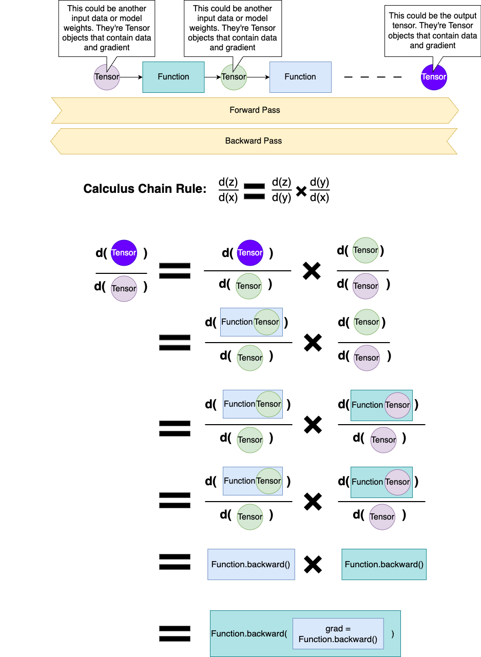
Figure 3
Tensor.backward()
One special tensor-level operation is the backward(). Note that this is different from the Function.backward().
Function.backward()computes the local partial derivative for a given function in the computational graph,Function.backward()is called by the library, never by the user.Tensor.backward()is the top-level entry point for backward propagation of the graph. In the previous sections, we’ve talked about the basics of a neural network is to perform forward and backward propagation, right? In order to perform a backward propagation, you need to start from somewhere. Usually that’s from the output tensor or the loss tensor if we computed a loss (refresher).
When you call Tensor.backward(), you’re computing the gradient of that final tensor with respect to all the tensors that led to it in the computational graph. For example, if z = f(y) and y = g(x), we must backward pass from z into y before we backward pass from y into x. This matches the classic post-order traversal algorithm, where we visit all of a node’s children before visiting that node. We will implement this using depth-first search (DFS) in post-order manner.
Why pre-order traversal is not enough: In a graph where one node depends on multiple inputs, you’d need all child gradients merged into the parent. But if pre-order visits the parent first, the parent can’t properly collect the gradients from children that haven’t been visited yet.
Below is the implementation:
topological_sorted_tensors = []
visited = set()
stack = [(self, False)]  # node, has_visit_children

# Post-order traversal to figure out the order of the backprop
while stack:
  node, has_visit_children = stack.pop()
  if node not in visited:
    if not has_visit_children:
      # first time we see this node, push it again with has_visit_children=True
      stack.append((node, True))
      # then push its parents
      if node.creator is not None:
        for p in node.creator.tensors:
          if p.requires_grad:
            stack.append((p, False))
    else:
      # Now we've visited node's inputs (second time seeing node),
      # so node is in correct post-order
      visited.add(node)
      topological_sorted_tensors.append(node)
We start off with the final output tensor (self) whose .backward() was called and we initialize the stack with (self, False). The reason we use a stack, as opposed to a recursion solution, is to avoid very large graphs creating large recursion stack and consuming lots of memory (the initial version was actually recursion).
We pop items off the stack. For each node (tensor):
- If we have not visited it yet and have not visited its children, we push
(node, True)back onto the stack. This signals that next time we pop it, we’ll treat it as “children done.” - We also push all of its parent Tensors (the inputs in
node.creator.tensors) onto the stack so they get visited first. - Eventually, once all children are visited, we pop
(node, True), and only then do we mark it as visited and add it totopological_sorted_tensors.
Below is the code for the actual backward propagation:
for tensor in reversed(topological_sorted_tensors):
  if tensor.creator is not None:
    grads = tensor.creator.backward(tensor.grad)
    for input_tensor, g in zip(tensor.creator.tensors, grads):
      if input_tensor is not None and input_tensor.requires_grad:
        input_tensor._accumulate_grad(g)
A depth-first search ensures each node’s children appear earlier in topological_sorted_tensors. If the graph looked like this x -> y -> z, then topological_sorted_tensors would contain [x, y, z] but we want to start backward propagation in [z, y, x] order, starting from the output tensor z. We will reverse the list.
- Compute local gradients (partial derivative) via
tensor.creator.backward(tensor.grad). Note thattensor.creatorwas assigned in our Function class apply() during forward pass. This calls theFunction.backward()specific derivative logic (e.g.MatMul.backward()). These refer to the blue and teal rectangle function boxes in Figure 3. - Accumulate those gradients into each input Tensor’s
.gradfield (input_tensor._accumulate_grad(g)), because multiple paths may flow into the same Tensor. - Free references (
tensor.creator.tensors = None) so we don’t hold onto the entire graph in memory.
That completes the entire backward pass (propagation) process from scratch. In the next section, I will go through some building blocks of neural networks (NN Module).
NN Module
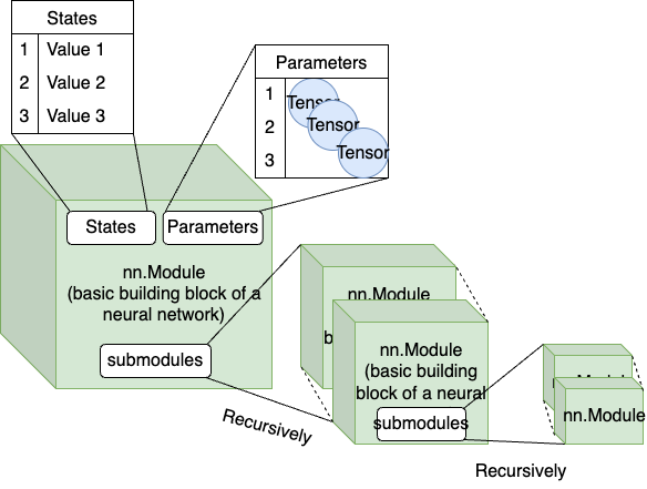
Figure 4
The main idea here is that we want to define the basic building block of a neural network – the nn.Module. We can later use this nn.Module class to define more complex neural network layers. This is the basis for any multi-layer perceptron, convolutional layers, recurrent layers, attention layers, all of which inherit from the basic nn.Module building block.
It’s important to take a look at the Module class skeleton (full code) to see what things are shared for all the neural network layers:
class Module:
  def __init__(self, *args, **kwargs):
    self._parameters: Dict[str, Tensor] = {}
    self._modules: Dict[str, "Module"] = {}
    self._states: Dict[str, Any] = {}
    self._is_training: Optional[bool] = None

  def zero_grad(self):
    # Zero gradients for parameters in current module
    for p in self._parameters.values():
        p.grad = 0

    # Recursively zero gradients in submodules
    for module in self._modules.values():
        module.zero_grad()

  @abstractmethod
  def forward(self, x) -> Tensor:
    raise NotImplementedError

  def train(self):
    for module in self._modules.values():
      module.train()
    self._is_training = True

  def eval(self):
    for module in self._modules.values():
      module.eval()
    self._is_training = False
- We can see this
Moduledefines an abstractforwardmethod. This needs to be implemented for all subclasses. Essentially, this function defines “how we transform the input Tensorxinto an output Tensor. It can be as simple asdef forward(self, x): return x + 1, but can also be more complicated. Anyways, this is the core of each neural network block. - We also see there are some instance variables such as
_parametersand_states._parametersstore the weights of the given neural network module/layer. Remember all weights are Tensor objects._statesare just arbitrary data that ann.Modulecan track. For example, a BatchNorm layer needs to track the running mean and variance for inference. - The
zero_gradfunction is used to clear out the gradients in all the weights in all the layers of the neural network before a new training iteration starts. Every iteration we will go through forward() and backward() to compute a fresh set of gradients for all the weights train/eval()help us to toggle the module/layer training mode on/off. This can be useful if a module/layer behaves differently, like in the Dropout layer
Where is backward()???
You might be wondering, we’ve always talked about each function should define its forward() and backward() in order for the computational graph to properly compute the gradients, and NN Module is essentially just another fancy function. You are 100% correct. So where is the backward() function?
Not defining the backward() here is intentional and is where the magic happens. Give me a minute, let me explain.
Remember that we are working with Tensor objects during the entire forward pass. And the forward pass is where we’re building the computational graph. As long as we perform Tensor-level operations, not NumPy operations, on Tensors, the library will correctly connect all the Tensors together from Tensor → Function → Tensor → Function → … → Tensor. Let’s take a look at the following example:
class DummyAdd(nn.Module):

  def __init__(self):
    super().__init__()
    self._parameters["weight"] = Tensor(data=np.array([0]))

  def forward(self, x, y):
    y2 = (y * self._parameters["weight"])
    z = x + y2
    return z

# y2.creator is Mul
# Mul.tensors = [y, self._parameters["weight"]]

# z.creator is Add
# Add.tensors = [x, y2]
# z.creator.tensors = [x, y2]
Now the question is, do we need to define the backward() for this DummyAdd module? Let’s try to call z.backward() without defining it.
In [6]: x = Tensor(10)
   ...: y = Tensor(20)
   ...: z = DummyAdd().forward(x, y)
In [7]: z
Out[7]: Tensor(data=[10.], grad=None)
In [8]: z.backward()
In [9]: z
Out[9]: Tensor(data=[10.], grad=Tensor(data=[1.], grad=None))
How come there’s no error? And how was z.grad computed?
This is the magic of Tensor-level operations. We have implemented the forward() and backward() of Add and Mul, which are called by __add__ and __mul__, triggered by the + and * in our DummyAdd.forward(). And the computational graph was built during the forward pass. Therefore, we don’t need to define a backward() function in the nn.Module anymore! Note that I highlighted that “As long as we perform Tensor-level operations, not NumPy operations, on Tensors …”. Performing NumPy operations will break this computational graph. See the example below
class DummyAdd(nn.Module):
  ...
  def forward(self, x, y):
    y2 = (y * self._parameters["weight"])
    z = np.sqrt(x + y2)
    return z
z now is constructed by np.sqrt, but np.sqrt doesn’t know how to do backward(), so z.backward() will not back propagate the gradient calculations to the input x and y. That’s why for anything that’s used in the module/layers, we need to implement the Tensor-level operations following the Function class interface. As of this writing, I have implemented the most common 23 tensor-level operations in tensor.py, necessary to tackle basic regression, computer vision, and natural language processing problems.
In short, nn.Module lays the foundation for building an entire neural network from smaller blocks (e.g. Linear module). Other complex layers just inject more complex logic into the forward(), or track some internal states. There’s nothing too scary. The famous “Attention is All You Need” (paper) attention mechanism is implemented like this using this library.
Functional Module
If you followed along, you might have already noticed the example in the Comparing this project to PyTorch for the same functionality section has already provided a flavor of what functional modules look like.
In this module, we basically implement some activation functions (e.g. ReLU, Softmax, Tanh, Sigmoid, etc) and loss functions (e.g. cross-entropy). Since they are functions, they also are subclasses of the Function class, similar to the tensor operations. If you have followed along, you would know the core of functions are forward() and backward(). I won’t paste any code examples, since they are very similar to any other function that we’ve shown above. If interested, check out the functional.py full code.
Optimizer
This module basically helps us update the weights of the neural network. In the most basic form, we have an optimizer class. And this optimizer class knows how to update the weights and incorporates the concept of a learning rate. There are some popular optimizers such as Stochastic Gradient Descent (SGD) and Adam. These are specific implementations of an optimizer. Certain optimizers might have different characteristics such as different learning rate schedules or additional states that they’re tracking. For example the Adam optimizer tracks “momentum” in addition to the normal learning rate. If interested, check out the optim.py full code.
class Optimizer:
  def __init__(self, model_parameters, lr):
    self._hyperparams: Dict[str, Any] = {}
    self._states: Dict[str, Any] = defaultdict(dict)

    self.model_parameters = model_parameters
    self._hyperparams["lr"] = lr

  def zero_grad(self):
    for k, module in self.model_parameters.items():
        for param_name, param in module.items():
            param.grad = None

  def step(self):
      """
      Performs a single optimization step.
      """
      raise NotImplementedError
If we look at the above code:
model_parameters: The layers or weights of the model are passed into theOptimizer(model_parameters). The Optimizer can then iterate over these parameters to update their values based on the gradients in thestep()- Hyperparameters and States
_hyperparams: Stores things like the learning rate (lr), or momentum factors, \(\beta_1, \beta_2\) for Adam, etc._states: For certain optimizers (like Adam or RMSProp), we need to maintain running estimates (e.g. first or second moments of gradients). Thisdefaultdictis where we can keep track of that “internal memory” keyed by state name.
zero_grad: Clears out any existing gradients in all the parameters before we compute new ones in a fresh forward/backward pass. This prevents mixing gradients from multiple batches. Obviously, this is an oversimplified example, because we could have arbitrary nested “model/layers/modules”.step: The core logic for updating parameters should be defined here. Each specialized optimizer (e.g. SGD, Adam) overrides step() to implement its update rule. A simple SGDstep()might look like thisparam.data = param.data - lr * param.grad.data.
That’s it. We’ve covered the core functionalities of a machine learning library.
Additional Thoughts
This section contains some thoughts I had while working on this project:
- Library: Creating a library from scratch requires careful design decisions along the way (e.g., how to represent data, which levels of abstraction to introduce, and how to balance speed of prototyping vs. generalization). Each choice can ripple through the entire codebase, so it’s important to stay flexible and open to refactoring.
- Importance of Unit Tests: Maintaining robust, near-100% test coverage ensures that adding new features or tweaking interfaces (e.g.,
FunctionorTensor) won’t break existing functionality. This gives me confidence to experiment and refactor without fear of introducing hidden bugs, which is very necessary when developing library from scratch. - Debugging Neural Networks: Neural networks are challenging to debug due to their arbitrary high-dimensional parameter spaces. Comparing gradients against PyTorch’s outputs, quickly overfitting on small datasets, and nudging weights manually helps identify and fix issues in both forward and backward passes.
- Performance Testing: Since the focus of this project is on education rather than library efficiency, I created a simple performance test script to ensure memory and CPU usage have not regressed. It helped me make the Tensor operation migration from the “closure” approach to
Functionclass smooth as butter. - Documentation: I’ve set up a ReadtheDocs page which provides a good overview of the latest APIs and features implemented in the library. Note that the examples I’ve included in this post are very bare-bones to just illustrate a point. The full functionality of the library is more powerful than that. Feel free to check it out or reference the doc to build your next toy model using this library.
- Example models: It’s important to create example models using this library, which help find blind spots and create motivation for me to keep adding new functionality to the library. Feel free to check them out in the examples/ (including GPT-2). These examples demonstrate both how the library can be used and its capability to build and train real-world models from scratch.
- In-place operations are tricky to implement: In-place operations like
+=and*=can save memory but are difficult to implement in a dynamic computational graph. Ensuring gradient correctness while avoiding data copies remains a challenge. Currently, I haven’t fully implemented gradient tracking for arbitrary in-place slicingmatrix[:, 1:10, :] += new_value, so we have to useslice1 = matrix[: 1:10], slice2 = matrix[:, 11:20] Tensor.cat([slice1, slice2]). - Derivative: Computing the derivative of every Tensor/activation/loss function can be tedious. This complexity can be compounded by broadcasting and shape mismatches. But once you have them implemented, the magic happens when you don’t need to define the
backward()function for yournn.Modules.
Thanks a lot for reading this far. I hope you learned something new from this post and/or library. I know I did. This project was a rewarding deep dive into the fundamentals of machine learning and library-building. Though it’s not optimized for large-scale training, it offers a flexible sandbox for experimenting with new techniques from papers or for random prototyping.