Code
1. Goal
The problem setting is to solve the Continuous MountainCar problem in OpenAI gym.

2. Environment
The mountain car follows a continuous state space as follows(copied from wiki):
The acceleration of the car is controlled via the application of a force which takes values in the range [1, 1]. The states are the position of the car in the horizontal axis on the range [1.2, 0.6] and its velocity on the range [0.07, 0.07]. The goal is to get the car to accelerate up the hill and get to the flag.
State
| Num | Observation | Min | Max |
|---|---|---|---|
| 0 | Car Position | -1.2 | 0.6 |
| 1 | Car Velocity | -0.07 | 0.07 |
Note that velocity has been constrained to facilitate exploration, but this constraint might be relaxed in a more challenging version.
Actions
| Num | Action |
|---|---|
| 0 | Push car to the left (negative value) or to the right (positive value) |
Reward
Reward is 100 for reaching the target of the hill on the right hand side, minus the squared sum of actions from start to goal.
This reward function raises an exploration challenge, because if the agent does not reach the target soon enough, it will figure out that it is better not to move, and won’t find the target anymore.
Note that this reward is unusual with respect to most published work, where the goal was to reach the target as fast as possible, hence favouring a bang-bang strategy.
Starting State
Position between -0.6 and -0.4, null velocity.
Episode Termination
Position equal to 0.5. A constraint on velocity might be added in a more challenging version.
The episode will terminate either when the car has reached the goal OR when the total number of time steps reached 1000 regardless of reaching the goal or not.
Solved Requirements
Get a reward over 90. This value might be tuned.
3. Approach
The approach uses the policy gradient algorithm with a baseline to reduce variance. Even though the state space is continuous, in this attempt, we will be using a discrete softmax policy. In other words, the continuous state space will be discretized into buckets of states that will be fed to the agent that will output a discrete action either [-1, 0, 1], which is [left, no-action, right].
3.1 Discretization
Since there are two dimensions in the state space, namely position and velocity. We will discretize them separately into 150 buckets and 120 buckets for position and velocity respectively.
3.2 Exploration vs Exploitation
To overcome the exploration-exploitation dilemma, we will be using the epsilon-greedy approach to slowly decrease the randomization factor overtime. This will ensure that our agent will have a wide variety of state-action training samples and in the later part of the training, it will allow the agent to follow it’s own “trained strategy” as opposed to random actions.
Technically, in the code, we will be using a temperature term to smooth the probability of actions, and epsilon to decide between whether to take a random action or the predicted action output from the policy.
3.3 Training
Monte Carlo
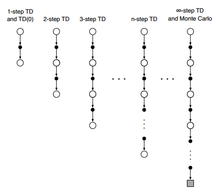
The training process follows a Monte Carlo method. This means the training only takes place after an entire episode is completed, and replays the accumulated state/action/reward/next state for training. This is at one end of the spectrum, the other end of the spectrum is called 1-Step Temporal Difference learning. So Monte Carlo is essentially a \(\infty\)-step Temporal Difference learning. There is a balance between when you want to train the agent. Training it too early could render very messy results and thus might be harder to converge. Training it too late might prolong the training duration for convergence. The criteria for choosing the method depends heavily on the problem itself.
Policy Gradient Weight Update \(\alpha_v = \text{Value function learning rate}\\ \alpha_p = \text{Policy function learning rate}\\ \hat{v} = \text{Estimated value for the given state} \\ \theta_v = \text{Value function parameterization weights}\\ \theta_p = \text{Policy function parameterization weights}\\ \delta = \text{Advantage}\\ \gamma = \text{Discount rate}\\\ G = \text{Discounted Rewards}\)
\[\Large \delta \leftarrow G - \hat{v}(S, \theta_{v})\\ \Large \theta_{v} \leftarrow \theta_{v} + \alpha_v \delta \triangledown \hat{v}(S, \theta_{v}) \\ \Large \theta_{p} \leftarrow \theta_{p} + \alpha_p \delta \gamma \triangledown \ln{\pi(A \mid S, \theta_p)}\\\]Gradient Calculation for Softmax Policy \(a = \text{action}\\ a' = \text{selected action by policy}\\ w = \text{policy weights}\\ \tau = \text{temperature for epsilon-greedy}\\ s = \text{current state} \\ \pi(a \mid s) = \text{policy outputs an action given the current state} \\ \Large \quad \quad \quad = \frac{e^{w_{s,a}}}{\sum_{a'}e^{w_{s,a'}}}\)
\[\Large \begin{align*} \triangledown_w \log \pi(a \mid s) &= \frac{\partial \log \frac{e^{w_{s,a}} / \tau}{\sum_{a'}e^{w_{s,a'}} / \tau}}{\partial w} \\ \newline \\ \text{(Take logs)} \; &= \frac{\partial \log \big(e^{w_{s,a}} / \tau\big) - \partial \log \big (\sum_{a'}e^{w_{s,a'}} / \tau \big)} {\partial w}\\ \newline \\ \text{(Chain & Log rule)} &= \frac{e^{w_{s, a}} / \tau w_{s,a} / \tau}{e^{w_{s,a}} / \tau \ln{e}} - \frac{\sum_{a'} w_{s,a'} / \tau \; e^{w_{s,a'}/ \tau}}{\sum_{a'}e^{w_{s,a'}}/ \tau}\\ \newline \\ \text{(Simplify first equation)} \; &= w_{s,a} / \tau - \frac{\sum_{a'} w_{s,a'} / \tau \; e^{w_{s,a'}/ \tau}}{\sum_{a'}e^{w_{s,a'}}/ \tau}\\ \newline \\ % \text{(Second equation substitute } \pi(a \mid s) \text{)} \; &= w_{s,a} / \tau - \sum_{a'} w_{s,a'} / \tau \; \pi(a' \mid s)\\ \text{(If Action = $a^\prime$) } &= (1 - \frac{e^{w_{s, a}}}{\sum_{a'}e^{w_{s,a'}}}) / \tau \\ &= \frac{1 - \pi(a \mid s)}{\tau} \\ \text{(If Action $\neq a^\prime$) } &= -(\frac{e^{w_{s, a}}}{\sum_{a'}e^{w_{s,a'}}}) / \tau \\ &= - \frac{\pi(a \mid s)}{\tau} \\ \end{align*}\]3.4 Hyperparameters
- Discount rate (\(\gamma\)): 0.999
- Value function learning rate (\(\alpha_v\)): \(1e^{-2}\)
- Policy function learning rate (\(\alpha_p\)): \(1e^{-3}\)
- Temperature (\(\tau\)): 1 decreasing to 0.5 linearly over all training episodes
- Discretization for position state: 150 buckets
- Discretization for velocity state: 120 buckets
- Epsilon-greedy (\(\epsilon\)): 1 decreasing to 0.1 linearly over all training episodes
4. Experiment & Findings
| # Episodes | Training Time | Min. Reward | Max Reward |
|---|---|---|---|
| 2500 | 473 seconds | 31.7 | 90.6 |
| 1500 | 327 seconds | 31.5 | 89.9 |
| 1000 | 254 seconds | 31.2 | 89.3 |
| 500 | 154 seconds | 30.2 | 86.7 |
| 200 | 77 seconds | 31.1 | 84.6 |
4.1 Introducing baseline to reduce variance


The above comparison experiment is to show the effects of having a baseline on the agent’s performance. We can easily see from the rewards graph, the agent with baseline has a smaller variance in the rewards. This translates to a faster convergence rate.
4.2 Discrete vs Continuous Actions
This problem (MountainCarContinuous-v0) was intended to be solved using a continuous action policy. However, I didn’t use continuous actions because I wanted to see how well a discrete-action agent could perform on this simple task. In conclusion, the number of episodes until convergence is quite good. The overall max reward reaches the goal of 90 at around ~1000 episodes.
4.3 Performance
Let’s look at the leaderboard of this problem and MountainCar-v0, which is a discrete version of the problem.
| MountainCar-v0 | |
|---|---|
| User | Episodes before solve |
| Zhiqing Xiao | 0 (use close-form preset policy) |
| Keavnn | 47 |
| Zhiqing Xiao | 75 |
| Mohith Sakthivel | 90 |
| Anas Mohamed | 341 |
| Harshit Singh Lodha | 643 |
| Colin M | 944 |
| jing582 | 1119 |
| DaveLeongSingapore | 1967 |
| Pechckin | 30 |
| Amit | 1000-1200 |
| Gleb I | 100 |
| MountainCarContinuous-v0 | |
|---|---|
| User | Episodes before solve |
| Ashioto | 1 |
| Keavnn | 11 |
| camigord | 18 |
| Tobias Steidle | 32 |
| lirnli | 33 |
| khev | 130 |
| Sanket Thakur | 140 |
| Pechckin | 1 |
| Nikhil Barhate | 200 (HAC) |
This shows that our discrete policy is a good baseline to start with before we dive into continuous actions. With continuous actions, debugging might be slightly harder as the policy function will be slightly more complicated, perhaps using a neural network approximating the policy function.
5. Next Steps
An obvious next step would be to try out continuous actions on this same problem and see how much more “efficient” and “effective” training can be. Intuitively, with continuous actions, you would expect a more fine-grain control of the car, and thus less “bouncing” around. Think driving with full petal and full brake, it’s not a very effective way to drive, is it?
Another thing that could be interesting to try out is to change the “n” in the n-step Temporal Difference (TD) learning and see the effects with regards to performance, convergence rate, reward variance. Right now we are using Monte Carlo, which is essentially a \(\infty\)-step TD method.
The current approach uses policy gradient as the approach to train the agent. There are some limitations in policy-based methods. There are other reinforcement learning algorithms that can be used to tackle this problem such as Deep Q-Learning, and Actor-Critic. I will be tackling another OpenAI Gym problem (Pendulum-v0) using actor-critic. Stay tuned for my next post.